Machine learning and data science are being looked as the drivers of the next industrial revolution happening in the world today. This also means that there are numerous exciting startups looking for data scientists.  What could be a better start for your aspiring career!

However, still, getting into these roles is not easy. You obviously need to get excited about the idea, team and the vision of the company. You might also find some real difficult techincal questions on your way. The set of questions asked depend on what does the startup do. Do they provide consulting? Do they build ML products ? You should always find this out prior to beginning your interview preparation.

To help you prepare for your next interview, I’ve prepared a list of 40 plausible & tricky questions which are likely to come across your way in interviews. If you can answer and understand these question, rest assured, you will give a tough fight in your job interview.

Note: A key to answer these questions is to have concrete practical understanding on ML and related statistical concepts.

Interview Questions on Machine Learning

Q1. You are given a train data set having 1000 columns and 1 million rows. The data set is based on a classification problem. Your manager has asked you to reduce the dimension of this data so that model computation time can be reduced. Your machine has memory constraints. What would you do? (You are free to make practical assumptions.)

Answer: Processing a high dimensional data on a limited memory machine is a strenuous task, your interviewer would be fully aware of that. Following are the methods you can use to tackle such situation:

1. Since we have lower RAM, we should close all other applications in our machine, including the web browser, so that most of the memory can be put to use.
2. We can randomly sample the data set. This means, we can create a smaller data set, let’s say, having 1000 variables and 300000 rows and do the computations.
3. To reduce dimensionality, we can separate the numerical and categorical variables and remove the correlated variables. For numerical variables, we’ll use correlation. For categorical variables, we’ll use chi-square test.
4. Also, we can use PCA and pick the components which can explain the maximum variance in the data set.
5. Using online learning algorithms like Vowpal Wabbit (available in Python) is a possible option.
6. Building a linear model using Stochastic Gradient Descent is also helpful.
7. We can also apply our business understanding to estimate which all predictors can impact the response variable. But, this is an intuitive approach, failing to identify useful predictors might result in significant loss of information.

Note: For point 4 & 5, make sure you read about online learning algorithms & Stochastic Gradient Descent. These are advanced methods.

Q2. Is rotation necessary in PCA? If yes, Why? What will happen if you don’t rotate the components?

Answer: Yes, rotation (orthogonal) is necessary because it maximizes the difference between variance captured by the component. This makes the components easier to interpret. Not to forget, that’s the motive of doing PCA where, we aim to select fewer components (than features) which can explain the maximum variance in the data set. By doing rotation, the relative location of the components doesn’t change, it only changes the actual coordinates of the points.

If we don’t rotate the components, the effect of PCA will diminish and we’ll have to select more number of components to explain variance in the data set.

Know more: PCA

Q3. You are given a data set. The data set has missing values which spread along 1 standard deviation from the median. What percentage of data would remain unaffected? Why?

Answer: This question has enough hints for you to start thinking! Since, the data is spread across median, let’s assume it’s a normal distribution. We know, in a normal distribution, ~68% of the data lies in 1 standard deviation from mean (or mode, median), which leaves ~32% of the data unaffected. Therefore, ~32% of the data would remain unaffected by missing values.

Q4. You are given a data set on cancer detection. You’ve build a classification model and achieved an accuracy of 96%. Why shouldn’t you be happy with your model performance? What can you do about it?

Answer: If you have worked on enough data sets, you should deduce that cancer detection results in imbalanced data. In an imbalanced data set, accuracy should not be used as a measure of performance because 96% (as given) might only be predicting majority class correctly, but our class of interest is minority class (4%) which is the people who actually got diagnosed with cancer. Hence, in order to evaluate model performance, we should use Sensitivity (True Positive Rate), Specificity (True Negative Rate), F measure to determine class wise performance of the classifier. If the minority class performance is found to to be poor, we can undertake the following steps:

1. We can use undersampling, oversampling or SMOTE to make the data balanced.
2. We can alter the prediction threshold value by doing probability caliberation and finding a optimal threshold using AUC-ROC curve.
3. We can assign weight to classes such that the minority classes gets larger weight.
4. We can also use anomaly detection.

Know more: Imbalanced Classification

Q5. Why is naive Bayes so ‘naive’ ?

Answer: naive Bayes is so ‘naive’ because it assumes that all of the features in a data set are equally important and independent. As we know, these assumption are rarely true in real world scenario.

Q6. Explain prior probability, likelihood and marginal likelihood in context of naiveBayes algorithm?

Answer: Prior probability is nothing but, the proportion of dependent (binary) variable in the data set. It is the closest guess you can make about a class, without any further information. For example: In a data set, the dependent variable is binary (1 and 0). The proportion of 1 (spam) is 70% and 0 (not spam) is 30%. Hence, we can estimate that there are 70% chances that any new email would  be classified as spam.

Likelihood is the probability of classifying a given observation as 1 in presence of some other variable. For example: The probability that the word ‘FREE’ is used in previous spam message is likelihood. Marginal likelihood is, the probability that the word ‘FREE’ is used in any message.

Q7. You are working on a time series data set. You manager has asked you to build a high accuracy model. You start with the decision tree algorithm, since you know it works fairly well on all kinds of data. Later, you tried a time series regression model and got higher accuracy than decision tree model. Can this happen? Why?

Answer: Time series data is known to posses linearity. On the other hand, a decision tree algorithm is known to work best to detect non – linear interactions. The reason why decision tree failed to provide robust predictions because it couldn’t map the linear relationship as good as a regression model did. Therefore, we learned that, a linear regression model can provide robust prediction given the data set satisfies its linearity assumptions.

Q8. You are assigned a new project which involves helping a food delivery company save more money. The problem is, company’s delivery team aren’t able to deliver food on time. As a result, their customers get unhappy. And, to keep them happy, they end up delivering food for free. Which machine learning algorithm can save them?

Answer: You might have started hopping through the list of ML algorithms in your mind. But, wait! Such questions are asked to test your machine learning fundamentals.

This is not a machine learning problem. This is a route optimization problem. A machine learning problem consist of three things:

1. There exist a pattern.
2. You cannot solve it mathematically (even by writing exponential equations).
3. You have data on it.

Always look for these three factors to decide if machine learning is a tool to solve a particular problem.

Q9. You came to know that your model is suffering from low bias and high variance. Which algorithm should you use to tackle it? Why?

Answer:  Low bias occurs when the model’s predicted values are near to actual values. In other words, the model becomes flexible enough to mimic the training data distribution. While it sounds like great achievement, but not to forget, a flexible model has no generalization capabilities. It means, when this model is tested on an unseen data, it gives disappointing results.

In such situations, we can use bagging algorithm (like random forest) to tackle high variance problem. Bagging algorithms divides a data set into subsets made with repeated randomized sampling. Then, these samples are used to generate  a set of models using a single learning algorithm. Later, the model predictions are combined using voting (classification) or averaging (regression).

Also, to combat high variance, we can:

1. Use regularization technique, where higher model coefficients get penalized, hence lowering model complexity.
2. Use top n features from variable importance chart. May be, with all the variable in the data set, the algorithm is having difficulty in finding the meaningful signal.

Q10. You are given a data set. The data set contains many variables, some of which are highly correlated and you know about it. Your manager has asked you to run PCA. Would you remove correlated variables first? Why?

Answer: Chances are, you might be tempted to say No, but that would be incorrect. Discarding correlated variables have a substantial effect on PCA because, in presence of correlated variables, the variance explained by a particular component gets inflated.

For example: You have 3 variables in a data set, of which 2 are correlated. If you run PCA on this data set, the first principal component would exhibit twice the variance than it would exhibit with uncorrelated variables. Also, adding correlated variables lets PCA put more importance on those variable, which is misleading.

Q11. After spending several hours, you are now anxious to build a high accuracy model. As a result, you build 5 GBM models, thinking a boosting algorithm would do the magic. Unfortunately, neither of models could perform better than benchmark score. Finally, you decided to combine those models. Though, ensembled models are known to return high accuracy, but you are unfortunate. Where did you miss?

Answer: As we know, ensemble learners are based on the idea of combining weak learners to create strong learners. But, these learners provide superior result when the combined models are uncorrelated. Since, we have used 5 GBM models and got no accuracy improvement, suggests that the models are correlated. The problem with correlated models is, all the models provide same information.

For example: If model 1 has classified User1122 as 1, there are high chances model 2 and model 3 would have done the same, even if its actual value is 0. Therefore, ensemble learners are built on the premise of combining weak uncorrelated models to obtain better predictions.

Q12. How is kNN different from kmeans clustering?

Answer: Don’t get mislead by ‘k’ in their names. You should know that the fundamental difference between both these algorithms is, kmeans is unsupervised in nature and kNN is supervised in nature. kmeans is a clustering algorithm. kNN is a classification (or regression) algorithm.

kmeans algorithm partitions a data set into clusters such that a cluster formed is homogeneous and the points in each cluster are close to each other. The algorithm tries to maintain enough separability between these clusters. Due to unsupervised nature, the clusters have no labels.

kNN algorithm tries to classify an unlabeled observation based on its k (can be any number ) surrounding neighbors. It is also known as lazy learner because it involves minimal training of model. Hence, it doesn’t use training data to make generalization on unseen data set.

Q13. How is True Positive Rate and Recall related? Write the equation.

Answer: True Positive Rate = Recall. Yes, they are equal having the formula (TP/TP + FN).

Know more: Evaluation Metrics

Q14. You have built a multiple regression model. Your model R² isn’t as good as you wanted. For improvement, your remove the intercept term, your model R² becomes 0.8 from 0.3. Is it possible? How?

Answer: Yes, it is possible. We need to understand the significance of intercept term in a regression model. The intercept term shows model prediction without any independent variable i.e. mean prediction. The formula of R² = 1 – ∑(y – y´)²/∑(y – ymean)² where y´ is predicted value.   

When intercept term is present, R² value evaluates your model wrt. to the mean model. In absence of intercept term (ymean), the model can make no such evaluation, with large denominator, ∑(y - y´)²/∑(y)² equation’s value becomes smaller than actual, resulting in higher R².

Q15. After analyzing the model, your manager has informed that your regression model is suffering from multicollinearity. How would you check if he’s true? Without losing any information, can you still build a better model?

Answer: To check multicollinearity, we can create a correlation matrix to identify & remove variables having correlation above 75% (deciding a threshold is subjective). In addition, we can use calculate VIF (variance inflation factor) to check the presence of multicollinearity. VIF value <= 4 suggests no multicollinearity whereas a value of >= 10 implies serious multicollinearity. Also, we can use tolerance as an indicator of multicollinearity.

But, removing correlated variables might lead to loss of information. In order to retain those variables, we can use penalized regression models like ridge or lasso regression. Also, we can add some random noise in correlated variable so that the variables become different from each other. But, adding noise might affect the prediction accuracy, hence this approach should be carefully used.

Know more: Regression

Q16. When is Ridge regression favorable over Lasso regression?

Answer: You can quote ISLR’s authors Hastie, Tibshirani who asserted that, in presence of few variables with medium / large sized effect, use lasso regression. In presence of many variables with small / medium sized effect, use ridge regression.

Conceptually, we can say, lasso regression (L1) does both variable selection and parameter shrinkage, whereas Ridge regression only does parameter shrinkage and end up including all the coefficients in the model. In presence of correlated variables, ridge regression might be the preferred choice. Also, ridge regression works best in situations where the least square estimates have higher variance. Therefore, it depends on our model objective.

Know more: Ridge and Lasso Regression

Q17. Rise in global average temperature led to decrease in number of pirates around the world. Does that mean that decrease in number of pirates caused the climate change?

Answer: After reading this question, you should have understood that this is a classic case of “causation and correlation”. No, we can’t conclude that decrease in number of pirates caused the climate change because there might be other factors (lurking or confounding variables) influencing this phenomenon.

Therefore, there might be a correlation between global average temperature and number of pirates, but based on this information we can’t say that pirated died because of rise in global average temperature.

Know more: Causation and Correlation

Q18. While working on a data set, how do you select important variables? Explain your methods.

Answer: Following are the methods of variable selection you can use:

1. Remove the correlated variables prior to selecting important variables
2. Use linear regression and select variables based on p values
3. Use Forward Selection, Backward Selection, Stepwise Selection
4. Use Random Forest, Xgboost and plot variable importance chart
5. Use Lasso Regression
6. Measure information gain for the available set of features and select top n features accordingly.

Q19. What is the difference between covariance and correlation?

Answer: Correlation is the standardized form of covariance.

Covariances are difficult to compare. For example: if we calculate the covariances of salary ($) and age (years), we’ll get different covariances which can’t be compared because of having unequal scales. To combat such situation, we calculate correlation to get a value between -1 and 1, irrespective of their respective scale.

Q20. Is it possible capture the correlation between continuous and categorical variable? If yes, how?

Answer: Yes, we can use ANCOVA (analysis of covariance) technique to capture association between continuous and categorical variables.

Q21. Both being tree based algorithm, how is random forest different from Gradient boosting algorithm (GBM)?

Answer: The fundamental difference is, random forest uses bagging technique to make predictions. GBM uses boosting techniques to make predictions.

In bagging technique, a data set is divided into n samples using randomized sampling. Then, using a single learning algorithm a model is build on all samples. Later, the resultant predictions are combined using voting or averaging. Bagging is done is parallel. In boosting, after the first round of predictions, the algorithm weighs misclassified predictions higher, such that they can be corrected in the succeeding round. This sequential process of giving higher weights to misclassified predictions continue until a stopping criterion is reached.

Random forest improves model accuracy by reducing variance (mainly). The trees grown are uncorrelated to maximize the decrease in variance. On the other hand, GBM improves accuracy my reducing both bias and variance in a model.

Know more: Tree based modeling

Q22. Running a binary classification tree algorithm is the easy part. Do you know how does a tree splitting takes place i.e. how does the tree decide which variable to split at the root node and succeeding nodes?

Answer: A classification trees makes decision based on Gini Index and Node Entropy. In simple words, the tree algorithm find the best possible feature which can divide the data set into purest possible children nodes.

Gini index says, if we select two items from a population at random then they must be of same class and probability for this is 1 if population is pure. We can calculate Gini as following:

1. Calculate Gini for sub-nodes, using formula sum of square of probability for success and failure (p^2+q^2).
2. Calculate Gini for split using weighted Gini score of each node of that split

Entropy is the measure of impurity as given by (for binary class):

Here p and q is probability of success and failure respectively in that node. Entropy is zero when a node is homogeneous. It is maximum when a both the classes are present in a node at 50% – 50%.  Lower entropy is desirable.

Q23. You’ve built a random forest model with 10000 trees. You got delighted after getting training error as 0.00. But, the validation error is 34.23. What is going on? Haven’t you trained your model perfectly?

Answer: The model has overfitted. Training error 0.00 means the classifier has mimiced the training data patterns to an extent, that they are not available in the unseen data. Hence, when this classifier was run on unseen sample, it couldn’t find those patterns and returned prediction with higher error. In random forest, it happens when we use larger number of trees than necessary. Hence, to avoid these situation, we should tune number of trees using cross validation.

Q24. You’ve got a data set to work having p (no. of variable) > n (no. of observation). Why is OLS as bad option to work with? Which techniques would be best to use? Why?

Answer: In such high dimensional data sets, we can’t use classical regression techniques, since their assumptions tend to fail. When p > n, we can no longer calculate a unique least square coefficient estimate, the variances become infinite, so OLS cannot be used at all.

To combat this situation, we can use penalized regression methods like lasso, LARS, ridge which can shrink the coefficients to reduce variance. Precisely, ridge regression works best in situations where the least square estimates have higher variance.

Among other methods include subset regression, forward stepwise regression.

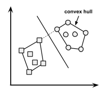
Q25. What is convex hull ? (Hint: Think SVM)

Answer: In case of linearly separable data, convex hull represents the outer boundaries of the two group of data points. Once convex hull is created, we get maximum margin hyperplane (MMH) as a perpendicular bisector between two convex hulls. MMH is the line which attempts to create greatest separation between two groups.

Q26. We know that one hot encoding increasing the dimensionality of a data set. But, label encoding doesn’t. How ?

Answer: Don’t get baffled at this question. It’s a simple question asking the difference between the two.

Using one hot encoding, the dimensionality (a.k.a features) in a data set get increased because it creates a new variable for each level present in categorical variables. For example: let’s say we have a variable ‘color’. The variable has 3 levels namely Red, Blue and Green. One hot encoding ‘color’ variable will generate three new variables as Color.Red, Color.Blue and Color.Green containing 0 and 1 value.

In label encoding, the levels of a categorical variables gets encoded as 0 and 1, so no new variable is created. Label encoding is majorly used for binary variables.

Q27. What cross validation technique would you use on time series data set? Is it k-fold or LOOCV?

Answer: Neither.

In time series problem, k fold can be troublesome because there might be some pattern in year 4 or 5 which is not in year 3. Resampling the data set will separate these trends, and we might end up validation on past years, which is incorrect. Instead, we can use forward chaining strategy with 5 fold as shown below:

• fold 1 : training [1], test [2]
• fold 2 : training [1 2], test [3]
• fold 3 : training [1 2 3], test [4]
• fold 4 : training [1 2 3 4], test [5]
• fold 5 : training [1 2 3 4 5], test [6]

where 1,2,3,4,5,6 represents “year”.

Q28. You are given a data set consisting of variables having more than 30% missing values? Let’s say, out of 50 variables, 8 variables have missing values higher than 30%. How will you deal with them?

Answer: We can deal with them in the following ways:

1. Assign a unique category to missing values, who knows the missing values might decipher some trend
2. We can remove them blatantly.
3. Or, we can sensibly check their distribution with the target variable, and if found any pattern we’ll keep those missing values and assign them a new category while removing others.

29. ‘People who bought this, also bought…’ recommendations seen on amazon is a result of which algorithm?

Answer: The basic idea for this kind of recommendation engine comes from collaborative filtering.

Collaborative Filtering algorithm considers “User Behavior” for recommending items. They exploit behavior of other users and items in terms of transaction history, ratings, selection and purchase information. Other users behaviour and preferences over the items are used to recommend items to the new users. In this case, features of the items are not known.

Know more: Recommender System

Q30. What do you understand by Type I vs Type II error ?

Answer: Type I error is committed when the null hypothesis is true and we reject it, also known as a ‘False Positive’. Type II error is committed when the null hypothesis is false and we accept it, also known as ‘False Negative’.

In the context of confusion matrix, we can say Type I error occurs when we classify a value as positive (1) when it is actually negative (0). Type II error occurs when we classify a value as negative (0) when it is actually positive(1).

Q31. You are working on a classification problem. For validation purposes, you’ve randomly sampled the training data set into train and validation. You are confident that your model will work incredibly well on unseen data since your validation accuracy is high. However, you get shocked after getting poor test accuracy. What went wrong?

Answer: In case of classification problem, we should always use stratified sampling instead of random sampling. A random sampling doesn’t takes into consideration the proportion of target classes. On the contrary, stratified sampling helps to maintain the distribution of target variable in the resultant distributed samples also.

Q32. You have been asked to evaluate a regression model based on R², adjusted R² and tolerance. What will be your criteria?

Answer: Tolerance (1 / VIF) is used as an indicator of multicollinearity. It is an indicator of percent of variance in a predictor which cannot be accounted by other predictors. Large values of tolerance is desirable.

We will consider adjusted R² as opposed to R² to evaluate model fit because R² increases irrespective of improvement in prediction accuracy as we add more variables. But, adjusted R² would only increase if an additional variable improves the accuracy of model, otherwise stays same. It is difficult to commit a general threshold value for adjusted R² because it varies between data sets. For example: a gene mutation data set might result in lower adjusted R² and still provide fairly good predictions, as compared to a stock market data where lower adjusted R² implies that model is not good.

Q33. In k-means or kNN, we use euclidean distance to calculate the distance between nearest neighbors. Why not manhattan distance ?

Answer: We don’t use manhattan distance because it calculates distance horizontally or vertically only. It has dimension restrictions. On the other hand, euclidean metric can be used in any space to calculate distance. Since, the data points can be present in any dimension, euclidean distance is a more viable option.

Example: Think of a chess board, the movement made by a bishop or a rook is calculated by manhattan distance because of their respective vertical & horizontal movements.

Q34. Explain machine learning to me like a 5 year old.

Answer: It’s simple. It’s just like how babies learn to walk. Every time they fall down, they learn (unconsciously) & realize that their legs should be straight and not in a bend position. The next time they fall down, they feel pain. They cry. But, they learn ‘not to stand like that again’. In order to avoid that pain, they try harder. To succeed, they even seek support from the door or wall or anything near them, which helps them stand firm.

This is how a machine works & develops intuition from its environment.

Note: The interview is only trying to test if have the ability of explain complex concepts in simple terms.

Q35. I know that a linear regression model is generally evaluated using Adjusted R² or F value. How would you evaluate a logistic regression model?

Answer: We can use the following methods:

1. Since logistic regression is used to predict probabilities, we can use AUC-ROC curve along with confusion matrix to determine its performance.
2. Also, the analogous metric of adjusted R² in logistic regression is AIC. AIC is the measure of fit which penalizes model for the number of model coefficients. Therefore, we always prefer model with minimum AIC value.
3. Null Deviance indicates the response predicted by a model with nothing but an intercept. Lower the value, better the model. Residual deviance indicates the response predicted by a model on adding independent variables. Lower the value, better the model.

Know more: Logistic Regression

Q36. Considering the long list of machine learning algorithm, given a data set, how do you decide which one to use?

Answer: You should say, the choice of machine learning algorithm solely depends of the type of data. If you are given a data set which is exhibits linearity, then linear regression would be the best algorithm to use. If you given to work on images, audios, then neural network would help you to build a robust model.

If the data comprises of non linear interactions, then a boosting or bagging algorithm should be the choice. If the business requirement is to build a model which can be deployed, then we’ll use regression or a decision tree model (easy to interpret and explain) instead of black box algorithms like SVM, GBM etc.

In short, there is no one master algorithm for all situations. We must be scrupulous enough to understand which algorithm to use.

Q37. Do you suggest that treating a categorical variable as continuous variable would result in a better predictive model?

Answer: For better predictions, categorical variable can be considered as a continuous variable only when the variable is ordinal in nature.

Q38. When does regularization becomes necessary in Machine Learning?

Answer: Regularization becomes necessary when the model begins to ovefit / underfit. This technique introduces a cost term for bringing in more features with the objective function. Hence, it tries to push the coefficients for many variables to zero and hence reduce cost term. This helps to reduce model complexity so that the model can become better at predicting (generalizing).

Q39. What do you understand by Bias Variance trade off?

Answer:  The error emerging from any model can be broken down into three components mathematically. Following are these component :

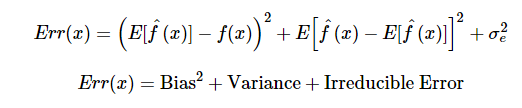
Bias error is useful to quantify how much on an average are the predicted values different from the actual value. A high bias error means we have a under-performing model which keeps on missing important trends. Variance on the other side quantifies how are the prediction made on same observation different from each other. A high variance model will over-fit on your training population and perform badly on any observation beyond training.

Q40. OLS is to linear regression. Maximum likelihood is to logistic regression. Explain the statement.

Answer: OLS and Maximum likelihood are the methods used by the respective regression methods to approximate the unknown parameter (coefficient) value. In simple words,

Ordinary least square(OLS) is a method used in linear regression which approximates the parameters resulting in minimum distance between actual and predicted values. Maximum Likelihood helps in choosing the the values of parameters which maximizes the likelihood that the parameters are most likely to produce observed data.

End Notes

You might have been able to answer all the questions, but the real value is in understanding them and generalizing your knowledge on similar questions. If you have struggled at these questions, no worries, now is the time to learn and not perform. You should right now focus on learning these topics scrupulously.

These questions are meant to give you a wide exposure on the types of questions asked at startups in machine learning. I’m sure these questions would leave you curious enough to do deeper topic research at your end. If you are planning for it, that’s a good sign.

Did you like reading this article? Have you appeared in any startup interview recently for data scientist profile? Do share your experience in comments below. I’d love to know your experience.

from:https://www.analyticsvidhya.com/blog/2016/09/40-interview-questions-asked-at-startups-in-machine-learning-data-science/